有限差分算例-Elliptic 方程求解#
本节将引导您使用 FEALPy 完成 Elliptic 方程的有差分求解,现定义如下数学模型:
\[\begin{split}
\begin{cases}
-\nabla (A \nabla u) + b \nabla u + c u = f & \text{在 } \Omega = [0,1]^2 \\
u = g & \text{在 } \partial \Omega
\end{cases}
\end{split}\]
其中我们定义真解为:
\[
u(x, y) = \sin(\pi x) \sin(\pi y)
\]
源项为:
\[
f(x,y) = (5\pi^2 + 4)\sin(\pi x) \sin(\pi y) + \pi \cos(\pi x) \sin(\pi y) - \pi \sin(\pi x) \cos(\pi y)
\]
系数为:
\[\begin{split}
A = \begin{pmatrix}
2 & 0 \\
0 & 3
\end{pmatrix}, \quad
b = \begin{pmatrix}
1 \\
-1
\end{pmatrix}, \quad
c = 4
\end{split}\]
1. 定义 PDE 模型#
from fealpy.backend import backend_manager as bm
from fealpy.decorator import cartesian

# 定义域
def domain():
    return [0, 1, 0, 1]

# 扩散项系数 A
def diffusion_coef():
    A = bm.tensor([[2.0, 0.0], [0.0, 3.0]])
    return A

# 对流项系数 b
def convection_coef():
    b = bm.tensor([1.0, -1.0])
    return b

# 反应项系数 c
def reaction_coef():
    return 4.0

# 真解
@cartesian
def solution(p):
    x = p[..., 0]
    y = p[..., 1]
    pi = bm.pi
    val = bm.sin(pi*x)*bm.sin(pi*y)
    return val

# 源项
@cartesian
def source(p):
    x = p[..., 0]
    y = p[..., 1]
    pi = bm.pi
    sin = bm.sin
    cos = bm.cos
    term1 = (5*pi**2 + 4) * sin(pi*x) * sin(pi*y)
    term2 = pi * cos(pi*x) * sin(pi*y)
    term3 = -pi * sin(pi*x) * cos(pi*y)
    val = term1 + term2 + term3
    return val

# dirichlet 边界条件
@cartesian
def dirichlet(p):
    return solution(p)
2. 进行参数配置和初始化#
设置后端
from fealpy.backend import backend_manager as bm

backend = 'numpy'
device = 'cpu'
bm.set_backend(backend)
导入日志工具
from fealpy.utils import timer
from fealpy import logger

logger.setLevel('WARNING')
tmr = timer()
next(tmr)
设置初始网格和加密次数
from fealpy.mesh import UniformMesh

mesh = UniformMesh(domain=domain(), extent=[0, 5, 0, 5])
maxit = 4
定义误差存储矩阵
errorMatrix = bm.zeros((1, maxit), dtype=bm.float64)
3. 有限差分求解#
流程包含:
(1)从离散格式组装刚度矩阵 \(A\) 和载荷向量 \(F\)
(2)处理 Dirichlet 边界条件
(3)求解线性系统 \(A u_h = F\)
(4)计算L2误差 \(\|u - u_h\|_{L^2(\Omega)}\)
(5)网格均匀加密
from fealpy.fdm import DiffusionOperator, ConvectionOperator, ReactionOperator, DirichletBC
from fealpy.solver import spsolve

for i in range(maxit):
    D = DiffusionOperator(mesh, diffusion_coef=diffusion_coef).assembly()
    C = ConvectionOperator(mesh, convection_coef=convection_coef).assembly()
    R = ReactionOperator(mesh, reaction_coef=reaction_coef).assembly()
    A = D + C + R

    node = mesh.entity("node")
    F = source(node)
    tmr.send(f'第{i}次矩阵组装时间')

    A, F = DirichletBC(mesh=mesh, gd=dirichlet).apply(A, F)
    tmr.send(f'第{i}次边界处理时间')

    uh = spsolve(A, F,solver='scipy')
    tmr.send(f'第{i}次求解器时间')
    errorMatrix[0, i] = mesh.error(solution, uh, errortype='L2')
    if i < maxit-1:
        mesh.uniform_refine(n=1)
    tmr.send(f'第{i}次误差计算及网格加密时间')
4. 误差分析和收敛阶计算#
next(tmr)
print("最终误差",errorMatrix)
print("order : ", errorMatrix[0,:-1]/errorMatrix[0,1:])
Timer received None and paused.
=================================================
   ID       Time        Proportion(%)    Label
-------------------------------------------------
    1     49.825 [ms]          76.996    第0次矩阵组装时间
    2      0.000 [us]           0.000    第0次边界处理时间
    3      3.351 [ms]           5.178    第0次求解器时间
    4    999.928 [us]           1.545    第0次误差计算及网格加密时间
    5      0.000 [us]           0.000    第1次矩阵组装时间
    6      1.017 [ms]           1.572    第1次边界处理时间
    7      0.000 [us]           0.000    第1次求解器时间
    8      0.000 [us]           0.000    第1次误差计算及网格加密时间
    9      1.001 [ms]           1.547    第2次矩阵组装时间
   10      0.000 [us]           0.000    第2次边界处理时间
   11    999.689 [us]           1.545    第2次求解器时间
   12      0.000 [us]           0.000    第2次误差计算及网格加密时间
   13      3.000 [ms]           4.635    第3次矩阵组装时间
   14    999.451 [us]           1.544    第3次边界处理时间
   15      3.518 [ms]           5.437    第3次求解器时间
   16      0.000 [us]           0.000    第3次误差计算及网格加密时间
=================================================
最终误差 [[0.00298339 0.00531285 0.00363034 0.00206084]]
order :  [0.56154201 1.46345801 1.76157855]
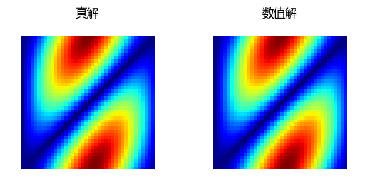
5. 结果可视化#
在单元重心处计算真解和数值解,并进行可视化比较
from matplotlib import pyplot as plt

node = mesh.entity('node')
u = solution(node)

fig, axes = plt.subplots(1, 2)
mesh.add_plot(axes[0], cellcolor=u, linewidths=0)
axes[0].set_title('真解', fontname='Microsoft YaHei')
mesh.add_plot(axes[1], cellcolor=uh, linewidths=0)
axes[1].set_title('数值解', fontname='Microsoft YaHei')
plt.show()