有限元算例-Poisson方程求解#
本节将引导您使用 FEALPy 完成 Poisson 方程的有限元求解,现定义如下数学模型:
\[\begin{split}
\begin{cases}
-\Delta u = f & \text{在 } \Omega = [0,1]^2 \\
u = g & \text{在 } \partial \Omega
\end{cases}
\end{split}\]
其中我们定义真解为:
\[
u(x, y) = \cos(\pi x)\cos(\pi y)
\]
源项为:
\[
f(x,y) = 2\pi^2 \cos(\pi x) \cos(\pi y)
\]
变分形式为:
\[
(\nabla u_h, \nabla v_h) = (f, v_h), \quad \forall v_h \in V_h
\]
1. 定义 PDE 模型#
from fealpy.backend import backend_manager as bm
from fealpy.decorator import cartesian

# 定义域
def domain():
    return [0, 1, 0, 1]

# 真解
@cartesian
def solution(p):
    x = p[..., 0]
    y = p[..., 1]
    pi = bm.pi
    val = bm.cos(pi*x)*bm.cos(pi*y)
    return val

# 源项
@cartesian
def source(p):
    x = p[..., 0]
    y = p[..., 1]
    pi = bm.pi
    val = 2*pi*pi*bm.cos(pi*x)*bm.cos(pi*y)
    return val

# dirichlet 边界条件
@cartesian
def dirichlet(p):
    return solution(p)
2. 进行参数配置和初始化#
设置后端
from fealpy.backend import backend_manager as bm

backend = 'numpy'
device = 'cpu'
bm.set_backend(backend)
导入日志工具
from fealpy.utils import timer
from fealpy import logger

logger.setLevel('WARNING')
tmr = timer()
next(tmr)
设置初始网格和加密次数
from fealpy.mesh import TriangleMesh

mesh = TriangleMesh.from_box(domain(), nx=4, ny=4)
maxit = 4
定义误差存储矩阵
errorMatrix = bm.zeros((1, maxit), dtype=bm.float64)
3. 有限元求解#
流程包含:
(1)构建Lagrange有限元空间
(2)组装刚度矩阵 \(A\) 和载荷向量 \(F\)
(3)处理Dirichlet边界条件
(4)求解线性系统 \(A u_h = F\)
(5)计算L2误差 \(\|u - u_h\|_{L^2(\Omega)}\)
(6)网格均匀加密
from fealpy.functionspace import LagrangeFESpace
from fealpy.fem import BilinearForm, ScalarDiffusionIntegrator
from fealpy.fem import LinearForm, ScalarSourceIntegrator
from fealpy.fem import DirichletBC
from fealpy.solver import cg

for i in range(maxit):
    space = LagrangeFESpace(mesh, p=1)
    tmr.send(f'第{i}次空间时间')
    uh = space.function()

    D = ScalarDiffusionIntegrator(q=3)
    bform = BilinearForm(space)
    bform.add_integrator(D)
    A = bform.assembly()
    lform = LinearForm(space)
    lform.add_integrator(ScalarSourceIntegrator(source, q=3))
    F = lform.assembly()
    tmr.send(f'第{i}次矩阵组装时间')
    gdof = space.number_of_global_dofs()
    A, F = DirichletBC(space, gd = dirichlet).apply(A, F)
    tmr.send(f'第{i}次边界处理时间')
    uh[:] = cg(A, F)
    tmr.send(f'第{i}次求解器时间')
    errorMatrix[0, i] = mesh.error(solution, uh)
    if i < maxit-1:
        mesh.uniform_refine(n=1)
    tmr.send(f'第{i}次误差计算及网格加密时间')
4. 误差分析和收敛阶计算#
next(tmr)
print("最终误差",errorMatrix)
print("order : ", bm.log2(errorMatrix[0,:-1]/errorMatrix[0,1:]))
Timer received None and paused.
=================================================
   ID       Time        Proportion(%)    Label
-------------------------------------------------
    1    594.125 [ms]          95.714    第0次空间时间
    2      6.998 [ms]           1.127    第0次矩阵组装时间
    3    995.398 [us]           0.160    第0次边界处理时间
    4      0.000 [us]           0.000    第0次求解器时间
    5      0.000 [us]           0.000    第0次误差计算及网格加密时间
    6      0.000 [us]           0.000    第1次空间时间
    7      1.609 [ms]           0.259    第1次矩阵组装时间
    8      0.000 [us]           0.000    第1次边界处理时间
    9      0.000 [us]           0.000    第1次求解器时间
   10      1.107 [ms]           0.178    第1次误差计算及网格加密时间
   11      0.000 [us]           0.000    第2次空间时间
   12      1.997 [ms]           0.322    第2次矩阵组装时间
   13      1.002 [ms]           0.161    第2次边界处理时间
   14      0.000 [us]           0.000    第2次求解器时间
   15      1.902 [ms]           0.306    第2次误差计算及网格加密时间
   16      0.000 [us]           0.000    第3次空间时间
   17      7.998 [ms]           1.288    第3次矩阵组装时间
   18      1.001 [ms]           0.161    第3次边界处理时间
   19    998.259 [us]           0.161    第3次求解器时间
   20      1.001 [ms]           0.161    第3次误差计算及网格加密时间
=================================================
最终误差 [[0.07186109 0.01940769 0.00495431 0.00124524]]
order :  [1.88858214 1.96987162 1.99225738]
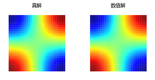
5. 结果可视化#
在单元重心处计算真解和数值解,并进行可视化比较
from matplotlib import pyplot as plt

bc = bm.array([[1/3, 1/3, 1/3]], dtype=bm.float64)
ps = mesh.bc_to_point(bc)
u = solution(ps)
uh = uh(bc)

fig, axes = plt.subplots(1, 2)
mesh.add_plot(axes[0], cellcolor=u, linewidths=0)
axes[0].set_title('真解', fontname='Microsoft YaHei')
mesh.add_plot(axes[1], cellcolor=uh, linewidths=0)
axes[1].set_title('数值解', fontname='Microsoft YaHei')
plt.show()